Tame your computer – make a break

Before I fell in love with Tables and PivotTables I regularly used Excel’s Outline functionality to group data and automatically insert subtotals and totals. OK, I might not use it for that purpose anymore, but if you’ve ever manually inserted page breaks when the content of a certain column changes, you might like to know you can do this automatically.

Here’s how:

1. Click any cell containing data you want to group and print on separate pages.
2. On the Data tab, click on the Sort A to Z or Sort Z to A button in the Sort & Filter group.
3. On the Data tab, click on the Subtotal button in the Outline group. (If the Subtotal button is greyed out you probably have your data formatted as a table. If so, click on the Convert to Range button in the Tools group on the Table Design tab to convert the table into a normal range of cells.)
4. From the At each change in drop-down list select the field you want to use for the page break. For example, Last Name or Product.
5. Select the Page break between groups check box.
6. Click OK.

Press CTRL + P to preview your print.

By the way, what I always liked about the Subtotal feature was that you can collapse and expand the worksheet to show various levels of your data.  For example, click on 1 to the left of column A to only see the grand total, 2 for grand total as well as subtotals and 3 for everything.

To remove the grouping, simply click on the Subtotal button and click on Remove All. (No, it won’t remove all; just the grouping. All of the data is preserved.)

Related tips

• Quickly format and enable filtering of your data
• Calculating subtotals and grand totals in a list

To help you put these tips into practice I have developed a series of 60-minute webinars, giving you the opportunity to see the hints, tips and time-saving shortcuts in action. And the price? £24. What are you waiting for?

Tame your computer – it’s a date

When you type, say, 16/2 in a cell, the default date format is typically 16-Feb. You can obviously quickly reformat the date using the Number Format drop-down button in the Number group on the Home tab and select Short Date or Long Date.

But talking about the dos and don’ts of working with Excel data (don’t use dots in dates), I was blown away by one of my webinar delegates last week who shared a keyboard shortcut to apply the dd-mmm-yy format. And as I am always on a hunt to do things easier and faster, I wanted to share her tip. (Thanks for the inspiration and your infectious enthusiasm during the two webinars, Heather!)

Here’s how:

1. Type the date. (Remember, you don’t have to type leading zeros and/or years.)
2. Select the cell(s) or column and press CTRL + #.

So if you press CTRL + ; (semicolon), select the cell and press CTRL + # today’s date is entered and formatted as 16-Feb-21.

By the way, looking for more information about this tip I find a lot of people saying you have to hold down the SHIFT key as well (i.e. press CTRL + SHIFT + #) but for me in various versions of Excel this doesn’t seem necessary. Anyone?

Oh, and to save  you time … no need to test that if you change your default Windows Region Settings that it changes what format CTRL + # applies … it doesn’t. It seems to be always using the dd-mmm-yy format, regardless of your default settings.

Related tips

• Insert today’s date or current time
• Format dates to include the day of the week
• Save time entering dates
• Enter the current date and/or time into a worksheet
• Convince Excel you want to type July 2010

That’s it for this week. And remember, to help you put these tips into practice I have developed a series of 60-minute webinars, giving you the opportunity to see the hints, tips and time-saving shortcuts in action. 24 pounds only!

Tame your computer – workbook wizardry

This week’s tip has been inspired by one of my delegates last week, who liked the idea of Quick Parts in Word and Outlook and asked whether it was also available in Excel. (Thanks for the inspiration, Sonal.)

Well, I’m afraid not, although you can vote for the feature to be added in future releases using the official Office 365 feedback and suggestions site here.

In the meantime, there are two alternatives you might want to check out …

Set up automatic text replacement using AutoCorrect – ideal for short pieces of text

Here’s how:

1.       On the File tab, click on Options.

2.       Click on Proofing or type the letter p.

3.       Click on the AutoCorrect Options button.

4.       In the Replace box, type a word or abbreviation you want to use as the “shortcut”. For example, KR.

5.       In the With box, type or paste your preferred text. For example, Karen Roem.

6.       Click Add.

7.       Click OK twice.

In Microsoft 365 the entries in the AutoCorrect list are available across all Office programs that support the AutoCorrect feature. So next time you type KR followed by a space or tab or carriage return, it will change KR to Karen Roem in Excel, Word, Outlook and PowerPoint.

Record a macro – ideal for pictures and longer text (It’s easier done than said and you only have to do this once!)

Here’s how:

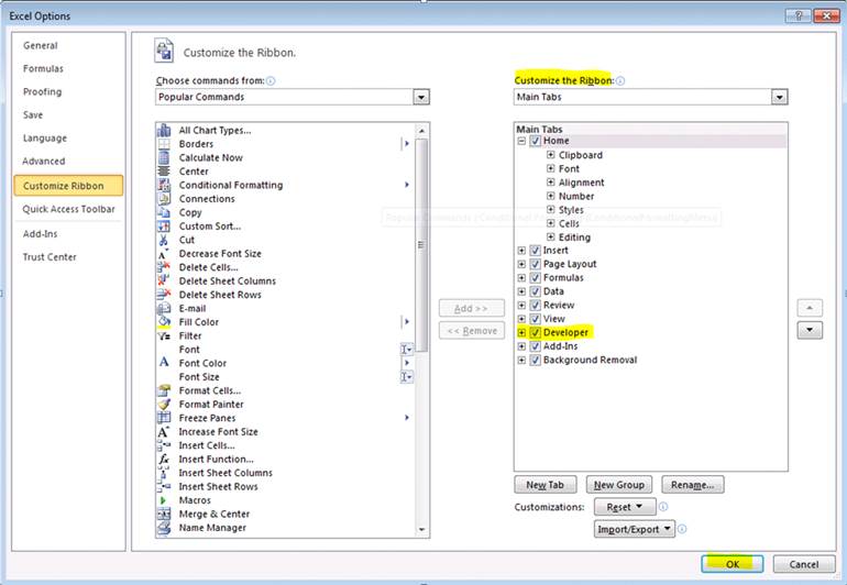
1.       If necessary, add the Developer tab to the ribbon by right-clicking anywhere on the Quick Access Toolbar and selecting Customize the Ribbon.

2.       On the Developer tab, in the Code group, click Record Macro.

3.       Type a name for the macro, such as autocorrect.

4.       Press TAB and hold down, say, the SHIFT key and type the letter A to assign CTRL + SHIFT + A as a keyboard shortcut to run the macro.

5.       Press TAB and select Personal Macro Workbook to make the macro available whenever you use Excel. (Make sure to click Save when you close down Excel and see a prompt to save the changes you made to the Personal Macro Workbook.)

6.       Press ENTER or click OK.

7.       Type the text and/or insert the picture you want to be able to insert as a reusable piece of content.

8.       On the Developer tab, in the Code group, click Stop Recording.

In future, you can use the shortcut key you assigned in step 4 to insert the text and/or picture. But why not check out tip 619 and add the macro as a button on your Quick Access Toolbar.

Related tips

• Create and modify Quick Parts to insert frequently used text, tables or pictures (Word and Outlook)
• Save and insert frequently used tables
• Create, store and insert frequently used text and graphics
• Create and insert frequently used text and graphics in Outlook
• Adding AutoCorrect Entries
• Open several workbooks with a single click

Tame your computer – Happy N(ew) Year

Hello and welcome to the first tip of 2021. Happy new year!

Speaking of new … do you use the File tab when you want to create a new document in Office? (That’s four clicks – not that I’m counting.) Or perhaps you click on the New button on the Quick Access Toolbar? (That is, if you stuck it on there.) Or perhaps you love keyboard shortcuts and use CTRL + N?

But did you know you can use this intuitive keyboard shortcut (the letter N for new) for so much more?

Here are some suggestions:

Word, Excel and PowerPoint : open a new document
Outlook : create a new email message or a meeting, contact or task – depending on what part of Outlook you’re in
Teams: start a new chat
Chrome and Edge : open a new browser window with cursor in address bar
Internet Explorer : open a copy of your current web page in a new window
Windows: open a copy of your current folder in a new window

By the way, on 1 January 2001 I turned my idea into reality and started my own business. So … happy 20th birthday to us. I would like to thank my clients for the opportunity to work on some amazing projects. And to my all-important course participants for choosing me to help tackle their time-consuming and frustrating day-to-day tasks. I wouldn’t be having a birthday if it wasn’t for you!

Related tips
Schedule your e-mail message to be sent at your preferred date and time (Microsoft Outlook)
Find the best time to schedule a meeting (Microsoft Outlook)
Open several workbooks with a single click (Microsoft Excel)

Tame your computer – FlashFill your case

As you probably know, Excel has no Change Case button like Word has. (And no, SHIFT + F3 doesn’t work either.) Instead, you might be using Excel’s UPPER and LOWER Functions to change text in a cell to UPPERCASE or lowercase.

But if you are using version 2013 or later you can use the Flash Fill functionality from the Auto Fill Options button that pops up when you’ve used the Auto Fill feature. Or – as described in tip 620 –  you can use its keyboard shortcut.

Here’s how:

1. Open FlashFill.zip to understand this example.
2. Click in cell B2.
3. Type ANNE BROWN or anne brown.
4. Press ENTER.
5. Press CTRL + E.

Excel will recognise the “pattern” you specified in step 3 and converts all text to uppercase or lowercase letters. No need to work with “helper columns” to store the newly formatted text. 

As a recent webinar attendee wrote “Like watching Professor McGonagall transfigure into a cat 🙂 “

Related tips
Split first name and last name into separate cells or combine first and last name in one cell
Quickly increase a list of numbers by one
Toggle between UPPER CASE, lower case and Sentence Case in Word

Upcoming courses
Given the new national lockdown restrictions, all our training sessions will be in a virtual setting from 5 November until 2 December. Our current course and webinar schedule can be found online.

Tame your computer – add Pivot power

If you have large amounts of information in Excel you probably (read: hopefully) use its powerful table management features to help you quickly retrieve and manipulate data. Perhaps you also use PivotTable reports to interactively summarize your data? Or maybe you’ve heard of PivotTables but never looked into them as yet? Or perhaps you don’t know what you don’t know?

Well you don’t have to … as long as you use version 2013 or later and your data has column headings, Microsoft will suggest a set of PivotTable reports it feels are most applicable.

Here’s how:

1. Click anywhere in your data.
2. On the Insert tab click on Recommended PivotTables (the second button from the left).
3. Use your downward arrow to flick through the various recommendations.
4. Click OK.

Your report has been inserted in a new sheet; your “raw data” is still intact and could be used as a basis for other summary reports.

Related tips
Quickly format and enable filtering of your data
See the data behind a specific figure in a PivotTable report
Filter data in a PivotTable and PivotChart using Slicers
Exclude data from your PivotTable report using Slicers

Two new webinars
Following the success of our four 60-minute webinars, I have developed two additional “further use” sessions, helping you to broaden your knowledge of Excel and Word and to benefit from its overlooked and underused features:

60-minute Further Use webinar – Excel with Excel 
Thursday 22 October, 10 – 11AM

60-minute Further Use webinar – Word to the wise  
Tuesday 27 October, 10 – 11AM

You can book your place online at the introductory price of  £24 per webinar per person. If you are looking for a webinar for a group of people, please get in touch.

And remember, as we respect the fact that people make special arrangements in their personal and professional lives for attending a session, we never cancel classes due to insufficient enrolments. Once payment is received, the webinar is guaranteed to run.

Tame your computer – name nudges

Have you ever needed to split a cell containing the full name of a person into a separate first name and last name cell? Perhaps you downloaded information from other software and you ended up with data in one cell that you would prefer to have in two cells?

If you are still using Excel 2010 you can use the Text to Columns option on the Data tab, as described in tip 225. But if you’ve upgraded to Excel 2013 or later you can use the Flash Fill functionality from the Auto Fill Options button that pops up when you’ve used the Auto Fill feature. (More about Auto Fill at the bottom of this tip under Related tips.)

But there is an even quicker way. OK, not a very intuitive one, but it’s so good I will remember!

Here’s how:

1. Open FlashFill.xlsx to understand this example.
2. Click in cell B2.
3. Type Anne.
4. Press ENTER.
5. Press CTRL + E.

You can also use it the other way around, i.e. turn two separate columns containing first name and last name into a full name. Much simpler than the CONCATENATE Function or the formula such as =A2&” “&B2.

With thanks to George for this week’s tip inspiration!

Related tips
Split first name and last name into separate cells
Move or copy cells using drag and drop
Stop AutoFill
Quickly increase a list of numbers by one
Quickly repeating a formula down a column
Quickly enter a series of weekdays

Upcoming webinars
The best way to understand Flash Fill and other tips is to see it in action. So why not sign up for one of our upcoming 60-minute webinars? (£20+VAT.)

As George wrote following his 60-minute Excel webinar … The course was really useful and worked well over video call. I would definitely recommend it to anyone wishing to brush up on their Excel knowledge.

Tame your computer – with mighty macros

When Microsoft released Excel 2013 it dropped one functionality that I really, really miss … Save Workspace, available in version 2010 in the Window group on the View tab. It allowed you to save several workbooks you needed for a particular task in a special workspace file  (*.xlw) so that when it was time to work on the job again, you just opened the workspace file and all files would be restored in the same arrangement you left them.

Like the idea? Why not record a macro that does just that? It might look daunting, but you only have to do this once and you can save yourself a lot of time in the long run.

Here’s how (in Excel 2013 and beyond):

1. If necessary, add the Developer tab to the ribbon by right-clicking anywhere on the Quick Access Toolbar and selecting Customize the Ribbon. Then, on the right hand side of the window,  tick the Developer check box under Main Tabs.
2. On the Developer tab, in the Code group, click Record Macro.
3. Type a name for the macro, such as workspace or several. (Avoid using the name Open.)
4. Press TAB and hold down, say, the SHIFT key and type the letter O to assign CTRL + SHIFT + O as a keyboard shortcut to run the macro.
5. Press TAB and select Personal Macro Workbook to make the macro available whenever you use Excel. (Make sure to click Save when you close down Excel and see a prompt to save the changes you made to the Personal Macro Workbook.)
6. Click OK.
7. Open the files you want be able to open in one go.
8. On the Developer tab, in the Code group, click Stop Recording.

In future, you can use the shortcut key you assigned in step 4 to open the various workbooks.

Bonus tip: why not add the macro as a button on your Quick Access Toolbar?

1. Right-click anywhere on the Quick Access Toolbar and select Customize Quick Access Toolbar.
2. In the Excel Options dialog box, under Choose commands from, click on Macros.
3. In the left list, double-click the newly created macro.
4. Press ENTER or click on the OK button.

By the way, you can still open a workspace (*.xlw) file that was created in an earlier version of Excel.

Upcoming 60-minute Excel webinars
Want to see these sort of Excel tips in action? Why not sign up for the next session planned for Tuesday 8 September 10:00 – 11:00 Book now
Price: £20 + VAT = £24

Related tips
Automating repetitive tasks
Customizing the Quick Access Toolbar
Selecting commands without using your mouse

Tame your computer – no half measures!

I cannot believe it’s July and we’re halfway through the year. And what a year it’s been so far. (The other day a friend of mine sent me a picture on WhatsApp stating “2020 – The year your wheelie bin goes out more than you.”) But I digress.

Inspired by halves and because I am keeping tabs on the hours I work from home for one of my clients I was looking for an easy way to round my numbers down to the nearest half. Excel has three Functions you might find helpful: FLOOR, CEILING, and MROUND.

Here’s how (click here to download an example in Excel):

1. Round down: =FLOOR(C2,.5) OR
2. Round up: =CEILING(C2,.5) OR
3. Round up or down: =MROUND(C2,.5)

You can also write 0.5 rather than .5 but you all know by now that I try to be as efficient as possible.

To make it look good, turn it into a table (CTRL + T) with totals (CTRL + SHIFT + T).

By the way, if you ever plan to hire me on a time and materials basis, don’t worry… I always round down 😉

Related tips
Quickly format and enable filtering of your data
Total the data in a table
Calculating a person’s age

Tame your computer – drop-down to validate your data

One of the ten dos and don’ts I always recommend to anyone who uses Excel as a database is “use data validation”. Whereas it can be used to reject invalid dates or to restrict the values that you can enter, I’ll kick this off describing a quick way to create a drop-down list containing specific text entries.

That way you can benefit from Excel’s powerful built-in tools to quickly summarise information, saving you countless hours consolidating, for example, inconsistent county entries such as Cambridgeshire, Cambs, CB etcetera.

Here’s how:

1. Select the cell(s) or column in which the restriction is to apply.
2. Click on the Data Validation button in the Data Tools group on the Data tab. (No need to click on its drop-down arrow.)
3. Expand the Allow box and select the List option.
4. Click in the Source box and type (or copy and paste) a list of entries, separated by commas. (For example: Bedfordshire, Berkshire, Buckinghamshire, Cambridgeshire, Cheshire, Cornwall, etcetera.)
5. Press ENTER.

In future, click on the drop-down arrow or use the ALT + down arrow trick I wrote about in May to select the appropriate entry from the drop-down list.

Finally, if you were wondering what the other nine of the ten dos and don’ts are …

1. Avoid empty rows and columns.
2. Do not merge cells.
3. Put your headings across columns, horizontally, rather than vertically.
4. Use separate columns for first name and last name.
5. Use dd/mm/yyyy date formats.
6. Do not immediately worry about sorting and formatting.
7. Put all raw data in one sheet instead of a sheet per month.
8. Use Excel Tables and pivot table reports and/or charts.
9. Add totals to a table.

By the way, if you want to know more about managing and summarising your data why not book an hour of virtual training? I’m using Zoom, which is easy to set up. If you’ve never used Zoom and are a bit worried we could run a quick, free test.

Alternatively, why not book yourself on the next half-day face-to-face session, planned for 7 August? See http://roem.co.uk/msexctables.php

Related tips

• Enter text from a list of previous entries
• Find and select data validation
• Total the data in a table
• Quickly format and enable filtering of your data